Introduction to the Python Overlay Network Graphical Simulator (PONGsim)
Abstract
This document describes PONGsim – a discrete-event simulator for simulating overlay networks such as those formed by peer-to-peer systems. The document describes how the existing simulations are used, the simulator structure, the fundamentals of extending the simulator and the main classes and methods.
1. Introduction
PONGsim is a discrete-event simulator for simulating overlay networks such as those formed by peer-to-peer systems. The simulator is implemented in the Python language [1], which allows for rapid prototyping with less time spent on coding. The philosophy behind the choice of language is that coding and experimenting should be quick, while the running time of the simulation is less important. The PONGsim framework allows implementation of new applications for generating overlay topologies and for performing searching and index distribution. PONGsim includes an implementation of the Search/Index Link (SIL) model [2].
1.1. Features
It has the following features:
- PONGsim is implemented in the Python language with emphasis on easy and rapid prototyping instead of runtime performance.
- PONGsim supports a batch mode and a graphical mode. The graphical mode is useful for prototyping and debugging new algorithms. The batch mode is useful for collecting statistics and evaluating how individual parameters affect the performance of an algorithm.
- PONGsim supports several instances to be run in parallel in batch mode. The instances select the following scenario from a common queue. The simulator controls the output files so that the output is not mixed between the instances. This is useful in computers with several processors or cores.
- PONGsim supports collection of statistics using several statistic tools.
- PONGsim allows easy definition of scenarios and access of scenario parameters from the code. Value ranges allow iterations of several values for a set of parameters.
- PONGsim supports repeating the same scenario multiple times and averaging the statistics.
- PONGsim supports adjusting the speed, allowing the operation to be examined in slow motion. Pausing allows individual simulation events to be run in steps. The redraw-interval in can be adjusted to allow a high speed also in the graphical mode.
- PONGsim uses a modular structure allowing easy implementation of new algorithms and architectures.
- PONGsim has short and fairly self-explanatory code with basic documentation.
- PONGsim implements a set of common unstructured peer-to-peer systems. Structured systems are currently under development.
1.2. History
PONGsim is based on the former simulator SNELSAN (Simple Network Layer Simulator for Ad-Hoc Networks) [3] used in the MobileMAN project of Helsinki University of Technology. The development of the simulator into an overlay simulator started in the MobileP2P project and continued during the Decicom project.
1.3. License
PONGsim is released [4] under MIT license.
2. Running simulations
This section gives a background for using the available simulations.
2.1. Understanding simulations
A simulation implements a system, situation or case that is analyzed. The simulation code invokes the simulator, which allows running the simulation with different parameters. Thus, the user selects which simulation is used already by running a specific simulation. For each simulation, several scenarios can be defined. A scenario is a set of parameters that are given as input to the simulation. Each scenario is defined in a scenario file. The scenario file is a list of parameter names and their corresponding values. A value can be a list of values, meaning that the simulator processes all values for that parameter in sequence. If the scenario file includes several parameters of list type, all possible combinations of parameter values are processed in sequence. Thus, a scenario file including a range represents several scenarios – one for each combination of range parameters.
2.2. Graphical mode
The simulator has a graphical mode and a batch mode. Starting the simulator without arguments invokes the graphical mode. The graphical user interface (GUI) consists of a graphical area reserved for displaying the network topology and a control area for displaying status information and controlling the simulation. Figure 1 shows an example of the graphical mode.
The graphical area to the left is controlled by the implementation of the current simulation. It allows a node to be selected in order to display information about the node. The node information is updated in real-time during simulations.
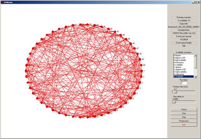
Figure 1. PONGsim window
The control area to the right shows the currently running scenario, the output file to which the statistics are collected, the current simulated time, the current simulation speed (events per second) and the current event queue length. The control area also includes the buttons, lists and sliders for controlling the simulation. The scenario list shows the available scenario files, from which the user can select the set of scenario files to be processed. Clicking a scenario name selects or deselects a scenario file. The run times –field allows the user to select how many times each scenario is repeated. This allows the same scenario to be run multiple times and averaging the results to reduce the statistical error. The redraw interval slider allows the user to adjust how often the graphical area is updated. A short update interval results in accurate display while a longer update interval increases the simulator speed. The step delay slider allows the user to control the simulator speed in order to slow down the simulator. It defines how long time the simulator waits after each simulated event. A speed of zero seconds is used for normal operation.
The buttons in the lower part of the control area control the execution of simulations. The run button starts a simulation sequence of the selected scenario files repeated the given number of times. When the simulator is running, the run button becomes a pause button, allowing a pause in the simulation. To continue after pausing, the user clicks the continue button. The stop button is used to interrupt the simulation and collect the statistics to the output file. The stop button clears the scenario queue. The scenarios and simulations can define stop criteria that stops a simulated scenario earlier, e.g. when the simulated time reaches a given value. After a scenario has finished, the following scheduled scenario will be started. The step button runs a single simulated event after which the simulator is paused. After running several scenarios, or after repeating a scenario several times, the user can click the postprocess button. This invokes a statistics processing function defined by the simulation code. Usually this averages the statistics of several simulator runs and creates tables from the collected data. The quit button exits the simulator application.
2.3. Batch mode
The batch mode is started when arguments are given on the command line. The first argument is the number of repetition per scenario. The rest of the arguments are file names of scenario files. The usage is thus:
python simulation.py repetition scenariofile1 [scenariofile2...]
The given scenarios are performed in sequence and repeated the given number of times.
2.4. Scenario file
The scenario file defines a list of parameters for a simulated scenario. A line in the parameter file is in the format
parameter=value
defining a value for a given parameter. The value can be an integer, a float, a Boolean or a string. A Boolean is defined as True or False. A string is given within quotation marks. A range can be defined as a set of values enclosed in braces:
parameter={value1 value2 value3}
A range creates a separate scenario for each of the given values, each simulated in sequence. If the parameter file has several range parameters, all possible combinations of values are simulated.
A special parameter is the file name of the output file given in the “file” parameter:
file=”simulation_with_[nodes]_nodes [runnumber].output.txt”
The file parameter can include other parameter values, so that these are inserted into the file name. These are given within brackets. When a scenario is repeated multiple times, the [runnumber] parameter gives the number of the current run, in order to create a separate output file for each run. Each scenario should generate a separate file, thus it is important that at least the range parameters are given in the file name to avoid overlapping file names.
2.5. Log file
The log file allows the operation of the simulation to be followed, which is especially valuable in batch mode. Each log file entry indicates the time, the type and a description of the logged event. When the simulation is running, also the simulated time is indicated. The type can be a warning, an error or some status information. New entries are appended to the log file, i.e. the file is not cleared when the simulator is started. Also the user can add information to the log file using the Log class.
2.6. Output file
The content of the output file is dependent of the implementation of the close() function in the Simulation class. Typically it contains the list of input parameters, a list of global counters and a collection of aggregated statistics.
During simulation the output file is locked using a file with the same name but with the “.lock” extension. This is used to indicate to other parallel processes that the given scenario is currently being simulated.
2.7. Postprocessing
Postprocessing can be performed when all simulated scenarios are performed. The postprocessing can be started using the user interface button or from the command line.
python simulation.py postprocess
The postprocessing is defined by the postprocess() function in the Simulation class. Typically postprocessing involves combining several runs and creating result tables. When a scenario is repeated several times, the runs can be combined with averaging to reduce statistical variation and dependence on given random number seeds. The table generator can create a set of tables based on selected output parameters and also perform simple calculations based on the output parameters.
3. Implementing simulations
This section gives a general overview of the simulator structure used for developing own simulations. The presentation includes only the most commonly used functions and classes.
3.1. Structure
The simulator is divided into several parts:
- Simulations implement a specific type of simulated case or situation that is evaluated.
- The main framework contains the infrastructure for simulating overlay networks. The main framework constitutes the critical part of the simulator which is included in all applications. It consists of a set of classes implementing the fundamental functions of the simulator.
- Additional features implement optional support to the simulator. Features include the Search/Index Link (SIL) model [2], a model of shared resources, a topology generator and a pseudo Bloom filter.
- Applications implement various overlay architectures and algorithms. Currently implemented are flooded searches, flooded index updates and the Direct Index algorithm [5].
- Utilities are used for processing statistics.
3.2. The simulator and the simulations
A simulation is implemented by extending the Simulation class. The task of the simulation is to create the nodes, connect nodes with links, attach applications to nodes, collect statistics and postprocess statistics.
The Simulation class defines the following functions.
- The __init__ standard python function is called when the Simulation class is created. It can be redefined provided that the __init__ of the superclass is called.
- The init function is called when a simulated scenario is started. Typically it creates the required counters, sets the random number seed, creates the nodes and the links and creates the resources.
- The close function is called when a simulated scenario is finished. Typically it reads the values from the counters and creates an output file.
- The eachevent function is called after each simulated event. Typically it checks whether the simulation should end, e.g. by comparing the current simulated time with some target time.
- The postprocess function is called when the user presses the postprocess button. Typically it averages the statistics from multiple runs and generates tables presenting the results.
The Simulator class manages the control of the simulation and the user interface. It creates a window with an area for the graphical view of the simulated network. It also shows the button used to control the simulations. The Simulator class should not be modified in normal cases.
The simulator is implemented by creating a Simulation object and a Simulator object. The Simulation object is passed as a parameter to the constructor of the Simulator object, together with the log file name and the directory containing the scenarios. Finally the run function of the Simulator is called to start the simulator. An example is the following:
mysimulation = MySimulation()
simulator = pongsim.Simulator(mysimulation,
“logfile.txt”, “scenarios/”)
simulator.run()
3.3. The main simulator framework
The main simulator framework defines the classes used by most simulations. It defines the following classes:
- The Scenario class stores the parameters of a simulated scenario. The most important functions are the following. The get(parameter) function returns the value of the indicated parameter. The format get(parameter, default) allows a default value to be given if the value is undefined by the user. The getname() function returns the name of the scenario. The getall() function returns a dictionary of all parameter values. The getfilename() function returns the filename used for this scenario. Converting a Scenario class to a string (using str) returns a representation of all parameter names and their values.
- The ScenarioManager loads and stores the scenarios, and manages the queue of scenarios to run. The user seldom needs to access this class.
- The Log class represents the log file. To write a line to the log, the warning(message), error(message) and status(message) functions are used. To write a line including the current simulated time to the log, the simwarning(message), simerror(message) and simstatus(message) functions are used.
- The Counter class allows counting events of different type. One Counter class contains several counter identified by their names. To add one to a named counter, the add(counter) function is called. To add a given value to a named counter, the add(counter, value) function is called. The Counter class can be activated and deactivated with the activate() and deactivate() functions, respectively. The add_override(counter, value) function can add values to a counter even if it is deactivated. Converting a Counter class to a string (using str) returns a representation of all counter names and their values. Giving a file name to the constructor reports all counter events to a file.
- The StatisticsCounter class implements a counter with better statistical capabilities. It calculates sum, max, min, average and the number of counted events. It is used like a Counter class but is slightly heavier. It returns the sum, average, entrycount, max and min with the sum(counter), average(counter), entrycount(counter), max(counter) and min(counter) functions. Also the string representation includes all information.
- The Snapshot class allows making periodical snapshots of the current simulated state.
- The EventQueue class is a priority queue used internally as the queue of scheduled simulated events.
- The Scheduler class manages the scheduled simulated events and the simulated time. The user schedules an event at a given simulated time by calling at(time, function, parameters). The event is given as a callback function with optional parameters. An event is scheduled after a given simulated delay with after(timedelay, function, parameters). A periodic event is scheduled with every(timeinterval, function, parameters). The current simulated time is obtained with the function time(). All times are given in simulated seconds.
- The Application class is the superclass for building applications. This is explained in detail in the following section.
- The Node class is the superclass for representing nodes. A node has a counter in Node.counter. The Node is related to a World class. A node can be assigned an address (in Node.address), or otherwise an address is generated automatically. A node’s positions in the graphical display is in the Node.x and Node.y coordinates. Also the node’s color and outline color can be assigned. The application running in a node is assigned with the setapplication(application) function. The existence of a node in the world can be checked with the inworld() function. Note that a Node class can exist even though it is not in the simulated world, thus, the simulator must on each event check whether the node is in the world. Sending and receiving messages is usually implemented through the Application class, thus the send and receive functions of the Node class are not directly used.
- The World class stores the nodes in a simulated world. Useful function include randomnode() to obtain a random node, randomcoordinate() to obtain a random coordinate in the world, getnodes() to get a list of all Node classes in the world, nodecount() to obtain the number of nodes, closest(x, y) to obtain the node closest to a given position.
- The Simulation class is the superclass for implementing simulations as described in the previous section.
- The StatusField class is a user-extendable display of various status information about the simulation. The function add(name, callback) allows an callback function to be registered, returning the value for the named status field.
- The Simulator class is the main simulator. Normal use does not require modifications to this class. The use is described in the previous section.
3.4. Applications
The modeled algorithms are implemented as applications by extending the Application class or alternatively by extending the SILApplication class.
The init() function is called when the application is initialized. The user can initialize various parameters and timers as well as resources when they are used.
For the graphical mode, the getdisplayinfo() function can be defined to return a text string (e.g. the address) shown beside the node. The getdetailedinfo() function can be defined to return a multi-line text string shown in a separate window when the node is selected. The draw(canvas, x, y) function can be defined to draw the node graphically on the given canvas at the given position. The default draw function draws the node as a circle.
The receive(message) function is called when the application receives a message. The send(message, destination) is used to send a message to the given destination address. Messages can be of any Python data type.
Note that in all callback functions of the application must test whether the node (and the application) currently exists:
if not self.node.world: return
3.5. Search/Index Link Applications
The pongsim_sil.SILApplication class extends the Application class with the Search/Index Link (SIL) model [2]. The SIL implementation defines the topology as a set of search and index links. It also includes a set of node-specific counters.
The init() function is called when the application is initialized. The user can initialize various parameters and timers as well as resources when they are used. The init() must call the superclass init() function.
A search link to a given destination address is created with addsearchlink(destination, ttl). The ttl is optional and indicates the default time-to-live value for search messages starting from this node. Index links are correspondingly created with addindexlink. Links can be removed using removesearchlink(destination) and removeindexlink(destination). Both additions can be combined with the addlink(destination, index, search, indexttl, searchttl) function.
To send a search message the floodsearch(message, ttl, id) function is used. If no ttl is specified, the link-specific one is used. If no id is specified, a random id is generated. An index message is sent correspondingly with floodindex. The messages are sent using the SIL model using flooding with a limited ttl. Other types of messages can be sent with sendgeneral(message, destination, type, ttl, id), whereas a specific destination is given. An optional type allows separating between several types of messages.
For receiving index messages the callback function receiveindex(ttl, message, destinations) is implemented. The ttl is the current ttl of the message. The destinations is a list of destinations to which the message will be forwarded. Normally the function ends with
return [(msg, destinations), ]
Thus, the same message is forwarded to the pre-evaluated destinations according to the SIL model. To implement other schemes the return value can be modified. The function must return a list of (message, destinations) tuples. Each tuple gives a message with a list of destination addresses to which the message is forwarded. The receivesearch function works in a similar way.
For receiving general messages the callback function receivegeneral(ttl, type, id, message) is implemented. The contents correspond to the sendgeneral function.
3.6. Modeling resources
Resources are modeled using the Resources class. Modeling includes the resource objects and the random requests to obtain resources. The Resources class also defines a set of node-specific counters.
The Resources class is initialized with
resources = Resources(log, searchinterval, indexaddinterval, indexremoveinterval, removeinitialresources, searchtimeout, dynamicresourcefrom, dynamicresourceto, postponeremoval, valuecounter)
The log is the Log class used for storing and displaying warning messages. The rest of the parameters give modeling parameters for resource usage. The searchinterval is the average interval between successive search requests. The indexaddinterval is the average interval between sucessive resource additions. The indexremoveinterval is the average time the resource is available at the node. The removeinitialresources is True if the initial resources should be removed after a indexremoveinterval. The searchtimeout is the time period after which the search results are examined. The dynamicresourcefrom is the start of the number range of resource numbers added dynamically. The dynamicresourceto is the end of the number range of resources added dynamically. The postponeremoval is True if removal of resources should be delayed until the following addition of resources. The valuecounter is a StatisticsCounter object that counts the delays and number of replies.
To use resources in an Application, the functions of the Resources class are inherited. Thus, both the Application (or SILApplication) and Resources are superclasses of the defined application. The application implements the following callback functions:
- on_added_resource(resource) is called when a random resource is added to the application. This may, for example, trigger an index update.
- on_removed_resource(resource) is called when a random resource is removed from the application. This may also, for example, trigger an index update.
- on_search_request(resource, searchid) is called when a search request is generated by the application. This typically triggers a search message. The searchid is used internally to pair requests and matched resources.
The local resources of a node are stored in the Node.localresources list. Thus, the application can check whether the requested resource is available locally. To count matches, the application reports the found resources using reportfound(searchid, where). The searchid is the same id as in the on_search_request function. The where parameter is the address of the node where the resource was found.
The AvailableResources class is simulator-wide register for the resources available at different nodes. It is used to assist searching so that a search will be directed to a resource that 1) exists and 2) is at any node. It is not normally used directly. However, it must be created as an object in the Simulator class:
mysimulator.availableresources = pongsim_resources.AvailableResources()
The node can be assign a set of initial resources with the initialresources(resources) function of the Resources class. To aid generating initial resources, the InitialResources class is available. It is initialized with the number of nodes. The generate(numberofresources, mincopies, maxcopies) function generates the given number of resources, each available in the given range of number of copies. The resources are obtained with the get() function, which can be given as parameter to the initialresources. The following example illustrates resource generation:
initialresources = pongsim_resources.InitialResources(len(nodes))
initialresources.generate(numberofresources, mincopies, maxcopies)
for node in nodes:
node.application.initialresources(initialresources.get())
3.7. Topology generator
The Topology class is used for generating random topologies. The constructor takes the number of nodes. The powerlaw_BA_degree(averagedegree) function generates a random power-law topology with the given average degree. The actually obtained average degree is available with the avgdegree() function. The isconnected() function returns True if the topology is connected. New topologies may be generated until a connected topology is obtained. The nodes in the generator is numbered. To get the list of neighbors of a given numbered nodes the neighbors(node) function is called.
3.8. Utilities
Utilities can be run as separate programs or as part of the postprocessing. Utilities include the pongsim_average and the pongsim_maketable utilities.
4. Conclusions
PONGsim provides a simulator framework that allows easy extensions for prototyping using the Python language. It contains simple functions for collecting statistics. It also has an implementation of the SIL model, which allows studies of more complex topologies. It allows resources to be modeled using a comprehensive set of parameters. Future developments include modeling of churn and implementation of structured peer-to-peer systems.